NSSO Series I: Reading National Sample Survey Data using R
I came across a nice talk by Sumandro (Riju) Chattopadhyay introducing National Sample Survey (NSS) data (link here). NSS data is distributed as fixed-width files, correctly referred to as the "Jurassic way" of data distribution by Riju.
Standard softwares can import fixed width format (fwf) files easily. In STATA, you can use infix or infile (used with a dictionary) commands to import. To read about ways to import NSS data in STATA, read this blog post by Zakaria Siddiqui.
In my first series of blogs, we will learn about ways to import, manage, visualize and analyze NSS data using R. To read fwf files in R, functions like read.fwf from base R can be used.
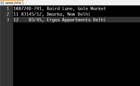
If we have a sample fwf file containg the following three rows of data and the layout as given below:

| VariableName | ColumnStart | ColumnEnd |
|---|---|---|
| SerialNumber | 1 | 2 |
| MonthlyIncome | 3 | 6 |
| Address | 7 | 36 |
We can import this file using the following R commands.
sample <- read.fwf("sample_fwf.txt", widths = c(2, 4, 30),
  col.names = c("sNo", "monthlyIncome", "address"), header = FALSE)
sample # print the sample file
  sNo monthlyIncome                        address
1  10          8724 D-741, Baird Lane, Gole Market
2  11           831       45/12, Dwarka, New Delhi
3  12            NA B5/45, Ergos Appartments Delhi
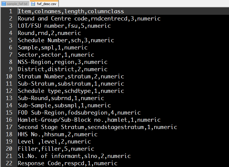
A possible way out to save you from the manual labor of typing out the column names and corresponding widths of large NSS data is to prepare a cleaner version of the layout file which can be imported using R. The clean layout file (screen-shot provided below) should contain the item description, byte length of the item, a short item description to be provided as column names and corresponding column classes as well, if needed.

This layout refers to Level 1 data of NSSO 66th Round Schedule 1.0 Consumer Expenditure Survey. The data distributed for this round has been arranged for different levels (there are 10 levels). Each block of the questionnare is linked to a level (multiple blocks can be part of the same level).
Now we have a clean layout file which can be directly read into R. The below commands can be used to import the fwf NSS data into R.
# import layout file
setwd("C:/Users/k.roy.chowdhury/Desktop/NSSO_v2/Class_26082015_Basics/Learning_R_Optional")
layoutFile <- read.csv("fwf_desc.csv", header = T)
head(layoutFile)
                   Item    colnames length columnclass
1 Round and Centre code rndcentrecd      3     numeric
2        LOT/FSU number         fsu      5     numeric
3                 Round         rnd      2     numeric
4       Schedule Number         sch      3     numeric
5                Sample        smpl      1     numeric
6                Sector      sector      1     numeric
# extract columns for arguments in read.fwf()
width <- as.vector(layoutFile$length)
columnNames <- as.vector(layoutFile$colnames)
columnClass <- as.vector(layoutFile$columnclass)
# read NSSO data
nssoLevel1 <- read.fwf("LVL66S0111.txt", widths = width, header = FALSE, col.names = columnNames, colClasses = columnClass)
head(nssoLevel1)
  rndcentrecd   fsu rnd sch smpl sector region district stratum substratum
1           1 84447  66  10    1      1     12        9       9          2
2           1 84447  66  10    1      1     12        9       9          2
3           1 84447  66  10    1      1     12        9       9          2
4           1 84447  66  10    1      1     12        9       9          2
5           1 84447  66  10    1      1     12        9       9          2
6           1 84447  66  10    1      1     12        9       9          2
  schdtype subrnd subsmpl fodsubregion hamlet secndstagestratum hhsnum
1        1      1       2          111      1                 1      1
2        1      1       2          111      1                 2      1
3        1      1       2          111      1                 2      2
4        1      1       2          111      1                 3      1
5        1      1       2          111      2                 1      1
6        1      1       2          111      2                 2      1
  level filler slno respcd svycd substncd datesvy datedispatch
1     1      0    1      2     1       NA  240909       151009
2     1      0    1      2     1       NA  220909       151009
3     1      0    1      2     1       NA  230909       151009
4     1      0    1      2     1       NA  240909       151009
5     1      0    1      2     1       NA  220909       151009
6     1      0    2      2     1       NA  210909       151009
  timetocanvass rmkbl1314 rmkelse spchok blank nss nsc    mlt
1           130         2       2     NA    NA   2   6  21185
2           130         2       2     NA    NA   2   6  66204
3           120         2       2     NA    NA   2   6  66204
4           130         2       2     NA    NA   2   6 132407
5           125         2       2     NA    NA   2   6 333666
6           125         2       2     NA    NA   2   6 444889
In the next post, we will learn how to automatically read all 10 level files with a single R function. See you soon!
References
- Sumandro Chattapadhyay; the aRt of NSSO data; URL http://www.slideshare.net/sumandro/sumandroanatomyofnssodataopendatacamp20120324
- Katyal, A. (et.al.); Using the Indian National Sample Survey data in public health research; The National Medical Journal of India, Vol. 26, No.5 (2013)
- Ray, S; Contribution of the National Sample Survey to Indian Agricultural Statistics; Journal of the Indian Society of Agricultural Statistics, Vol 59(1) (2005); URL http://isas.org.in/jsp/volume/vol59/sray.pdf